Classical Robotics in a Nutshell
Draft Author: Philipp Becker (philippbecker93@googlemail.com), Pascal Klink (pascal.klink@googlemail.com)
In this chapter we want to explore the foundations of robotics which we will need later in the course. But before we start, we should quickly think about the term 'robot'.
What is a Robot? 
Let's start with some examples. Most of us probably know the little fellow on the left and the brutal killing machine on the right:
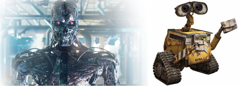 Figure 1: Some robot examples from Hollywood: A T-800 robot from the movie Terminator (left) and Wall-E (right)
However, we can also find lots of robots in reality - here a a few of them:
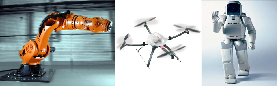 Figure 2: Real robot examples: An industrial robot (left), a quadrocopter (middle) and a humanoid robot (right)
While probably all of us would have agreed that all those above are robots, it may still be hard to tell what the essence behind the term 'robot' is. So let's see if some definitions may help us out here.
Definitions
We will first take a look at the classical industrial definiton of a robot:
A robot is a reprogrammable multifunctional manipulator designed to move material, parts, tools, or specialized devices through variable programmed motions for the performance of a variety of tasks. (Robotics Institute of America)
As we can see all the real and fictional robots from above fulfill the above criteria - for example the T-800 robot from Terminator can probably accomplish all the mechanical tasks a human can do and ever since Amazon announced his research on packet delivery by drones we know that quadrocopters can be used for autonomous aerial transportation tasks.
However, in this definition the robot is simply seen as just a factory element. But if you now picture Wall-E working double shifts in a car factory - don't panic! There are also more general definitions like the following:
A computer is just amputee robot. (G. Randlov)
Generally, we see a robot as a computer that can sense, plan and act in a physical environment.
Terminology
Now that we know what a robot is. Let's talk about the basic terminology we will need throughout this lecture. For that we will take a look at an Epson SCARA robot - which looks as follows:
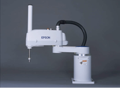 Figure 3: A scara assembly robot with two revolute joints and one prismatic joint
Joints, Links and Endeffectors
To be able to move - robots need joints just as we humans. The single joints of a robot are connected by so called links. An analogy from our body for two joints and a link between them is the knee joint and ankle which are connected by the shin. We can distinguish between two types of joints - revolute and prismatic joints:
 Figure 4: The representation of revolute and prismatic joints in 2D and 3D depictions of robots
As we can see, both types of joints have one degree of freedom. The difference between them is the kind of movement they are able to do - revolute joints rotate around a certain axis while prismatic joints move along it. The position of a revolute joint is described in radian while the position of a prismatic joint is described in meters.
The end effector of a robot is a device with which the robot interacts with its environment. End effectors are mostly placed at the end of robotic arms (just as it is the case for our SCARA robot) but this is not obligatory. For example, if you think of a quadrocopter a possible end effector could be a robotic claw which is fixed at the bottom of the quadrocopter.
Speaking about quadrocopters - as you may have already recognized quadropcopters do not have joints. You are absolutely right with that and indeed we need another method for describing robots of those kind (so called free floating robotics). However, we will not look at this in the lecture.
Now let's see what joints and links our SCARA robot has and where its end effector is:
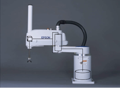 Figure 5: The scara assembly robot from above with a 3D depiction of its joints
State and Actions
As we know, joints give us the ability to move a robot. However in order to make the robot actually move - we need to tell him what to do. These commands are called actions. In general actions can be velocities, accelerations or torques/forces (depending on whether we have revolute or prismatic joints). However, in the field of robotics actions are always in some way mapped to torques/forces.
The state $\mathbf{s}(t)$ describes the configuration of the robot (which can be besides its joint positions also its application state) and it's environment for time $t$. Consequently, actions are the robots possibility to change the state by changing its joint positions.
Workspace
The workspace of a robot is the space it can reach with its end effector. For our SCARA robot this can (depending on the limits of the single joints) look as follows:
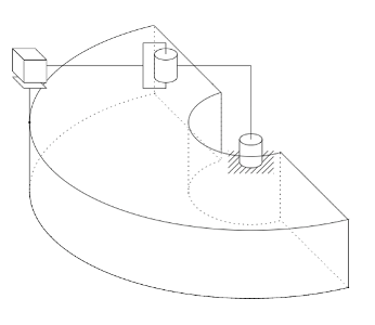 Figure 6: The workspace of the scara assembly robot from above
Joint- and Task space
As we know the state $\mathbf{s}(t)$ contains the joint positions of the robot. Often we are especially interested in the position of the end effector. This position can be described in two ways - either in the joint- or in the task space.
As the name indicates, we describe the end effector position in the joint space using a vector which contains all joint positions. For our SCARA robot this would correspond to the following vector:
$$\begin{align*} \mathbf{q}(t) = \begin{pmatrix}q_1(t)\\q_2(t)\\q_3(t)\end{pmatrix} \end{align*}$$In this case $q_1(t)$ corresponds to the first revolute joint position (the one at the bottom), $q_2(t)$ to the second revolute joint position (the one at the top) and $q_3(t)$ to the prismatic joint position at time $t$.
Describing the end effector in the task space can be done in many ways for one and the same robot, depending on how you choose to represent the environment of the robot. We could for example choose to represent it using cartesian coordinates but we could also use polar coordinates. If we choose the former we would use the following vector for our SCARA robot:
$$\begin{align*} \mathbf{x}(t) = \begin{pmatrix}x_1(t)\\x_2(t)\\x_3(t)\end{pmatrix} \end{align*}$$As you have probably already realised $x_1(t)$ is the x-, $x_2(t)$ the y- and $x_3(t)$ the z-coordinate of the end effector in the cartesian coordiante system at time $t$.
It is often also interesting to know about the orientation of our end effector. In the joint space we don't need to extend our vector, since the joint positions already tell us about the orientation of our end effector. In the task space we could for example use a second point in the cartesian coordinate system to indicate in which direction the end effector is oriented.
To make the formulas of the following chapters shorter, we will write $\mathbf{q}$ instead of $\mathbf{q}(t)$ and $\mathbf{x}$ instead of $\mathbf{x}(t)$
System Overview
Now enough with the terminology - let's look at the core components of a classical robot. For that let's first take a look at the following graphic:
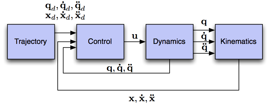 Figure 7: This figure shows the core elements of classical robotics. A desired trajectory consisting of positions, velocities and accelerations is either representated in task space by $\mathbf{x}_{d}$, $\mathbf{\dot{x}}_{d}$, $\mathbf{\ddot{x}}_{d}$, or in joint-space by $\mathbf{q}_{d}$, $\mathbf{\dot{q}}_{d}$, $\mathbf{\ddot{q}}_{d}$. Based on the desired trajectory and the current state of the robot in task-space $\mathbf{x}$, $\mathbf{\dot{x}}$, $\mathbf{\ddot{x}}$ or joint-space $\mathbf{q}$, $\mathbf{\dot{q}}$, $\mathbf{\ddot{q}}$, the control law generates a motor command $\mathbf{u}$ consisting of torques or forces. When these are applied to the robot, the state of the robot changes in joint-space as modeled by the dynamics and from that results a task-space change as modeled by the kinematics.
It is really key to remember the 4 components from above so here they go again with a short description for each one:
- Trajectory: Representation of your task.
- Control: Compute the motor commands you need to fulfill your task.
- Dynamics: Compute what your motor command would do to your robot.
- Kinematics: Convert joint space to task space.
We will now go through the single components and take a detailed look at them, starting off with kinematics and dynamics.
Kinematics 
So we know from above that we want to get from the representation of our robot in the joint-space to the representation of our robot in the task-space. The good news here is, it is a purely geometrical problem to solve. And if we use cartesian coordiates to represent our robot in task-space - which normally is the case - we basically only need trigonometry besides addition and multiplication to solve this problem (naturally the formulas can get quite cumbersome for robots with many joints).
In this chapter we will do the forward kinematics for the SCARA robot we already saw in figures 3 and 5.
Forwards Kinematics
First of all let's calculate the position in the task-space from the position in our joint-space. For that we need to define a function $f$ so that $\mathbf{x} = f(\mathbf{q})$. To do that it is best to make some sketches of the robot from various perspectives:
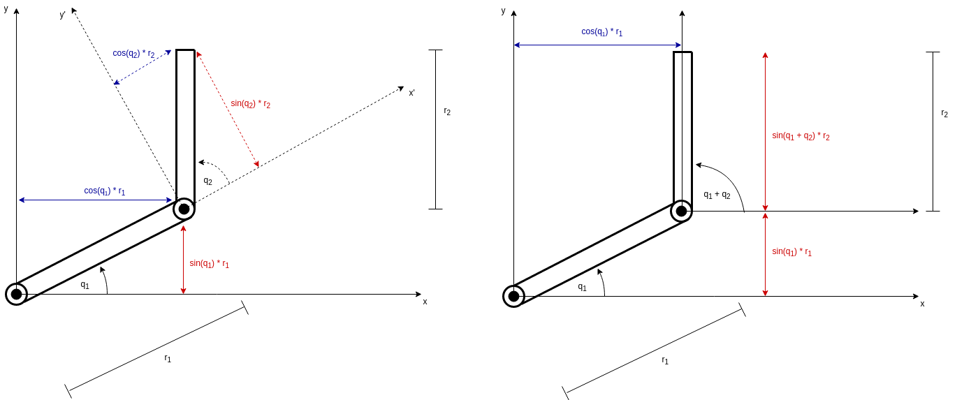 Figure 8: Sketches of the SCARA robot projected into the xy-plane - $q_1$ and $q_2$ are the positions of the two revolute joints (in rad) - $r_1$ and $_2$ are the lengths of the links between the joints (in meters)
We will start with calulcating the position of the robot arm in the xy-plane. As already pointed out in figure 8 we cannot just calculate $\cos(q_1) r_1 + \cos(q_2) r_2$ to calculate $x_1$ of our position vector $\mathbf{x}$. This is because the coordinate system in which we express the joint position $q_2$ is rotated according to the joint position $q_1$. So to measure the joint position in the actual coordinate system, we need to sum both rotations up. Considering this, our forward kinematics for the xy-plane will look as follows:
$$\begin{align*} \begin{pmatrix} x_1\\ x_2 \end{pmatrix} = \begin{pmatrix} \cos(q_1) r_1 + \cos(q_1 + q_2) r_2\\ \sin(q_1) r_1 + \sin(q_1 + q_2) r_2 \end{pmatrix} \end{align*}$$To finish the forward kinematics for our scara robot we will have to calculate the forward kinematics for the z-coordinate of the SCARA robot. Again we will first take a look at a sketch (this time it is not compliant to the joint representations from the chapter 'Terminology' - however, I could not come up with another good way of drawing it):
 Figure 9: A sketch of the SCARA robot projected into the xz-plane. $h_1$ and $h_2$ are the heights of the two revolute joints and $q_3$ is the position of the prismatic joint of the robot to which the end effector is connected
As we can see the forward kinematics for the z-coordinate of the robot is really easy. It is just $x_3 = h_1 + h_2 - q_3$. Bringing this all together we can now complete the forward kinematics for our SCARA robot:
$$\begin{align*} \begin{pmatrix} x_1\\ x_2\\ x_3 \end{pmatrix} = \begin{pmatrix} \cos(q_1) r_1 + \cos(q_1 + q_2) r_2\\ \sin(q_1) r_1 + \sin(q_1 + q_2) r_2\\ h_1 + h_2 - q_3 \end{pmatrix} \end{align*}$$Differential forward kinematics
So until now we defined $f(\mathbf{q})$ such that $\mathbf{x}=f(\mathbf{q})$. But if we again take a look at figure 7 we see that the control stage of a robot can also consume $\mathbf{\dot{x}}$ and $\mathbf{\ddot{x}}$. Luckily we can quite easily find functions $g(\mathbf{q}, \mathbf{\dot{q}})$ and $h(\mathbf{q}, \mathbf{\dot{q}}, \mathbf{\ddot{q}})$ sucht that $\mathbf{\dot{x}}=g(\mathbf{q}, \mathbf{\dot{q}})$ and $\mathbf{\ddot{x}}=h(\mathbf{q}, \mathbf{\dot{q}}, \mathbf{\ddot{q}})$ if we are familiar with differentiation and especially the chain rule for differentiation. With the latter we can derive the abstract form of our functions $g$ and $h$:
$$\begin{align*} \dot{\mathbf{x}} &= g(\mathbf{q}, \mathbf{\dot{q}}) = \frac{d(f(\mathbf{q}))}{dt} = \underset{\mathbf{J}\left(\mathbf{q}\right)}{\underbrace{\frac{df(\mathbf{q})}{d\mathbf{q}}}}\underset{\mathbf{\dot{q}}}{\underbrace{\frac{df(\mathbf{q})}{dt}}}= \mathbf{J}\left(\mathbf{q}\right)\mathbf{\dot{q}} \\ \ddot{\mathbf{x}} &= h(\mathbf{q}, \mathbf{\dot{q}}, \mathbf{\ddot{q}}) = \frac{d(g(\mathbf{q}, \mathbf{\dot{q}}))}{dt} = \frac{\mathbf{J}\left(\mathbf{q}\right)\mathbf{\dot{q}}}{dt} = \frac{\mathbf{J}\left(\mathbf{q}\right)}{dt}\mathbf{\dot{q}} + \mathbf{J}\left(\mathbf{q}\right)\frac{\mathbf{\dot{q}}}{dt} = \dot{\mathbf{J}}\left(\mathbf{q}\right)\mathbf{\dot{q}}+\mathbf{J}\left(\mathbf{q}\right)\mathbf{\ddot{q}} \end{align*}$$Note that $\dot{\mathbf{J}}\left(\mathbf{q}\right)=\frac{d\mathbf{J}(\mathbf{q})}{d\mathbf{q}} \mathbf{\dot{q}}$. Since we now have that, we can apply it to our Scara robot. However, we will just calculate the formula of $g$ here, since we need to work with tensors if we want to calculate $h$ (we need to calculate $\frac{d\mathbf{J}(\mathbf{q})}{d\mathbf{q}}$). Since we know that $\frac{d(\sin(x))}{dx} = \cos(x)$ and $\frac{d(\cos(x))}{dx} = -\sin(x)$ we get the following formula for $g$:
$$\begin{align*} g(\mathbf{q}, \mathbf{\dot{q}}) &= \mathbf{J}\left(\mathbf{q}\right)\mathbf{\dot{q}} \\ &=\begin{pmatrix} -\sin(q_1) r_1 - \sin(q_1 + q_2) r_2 & -\sin(q_1 + q_2) r_2 & 0 \\ \cos(q_1) r_1 + \cos(q_1 + q_2) r_2 & \cos(q_1 + q_2) r_2 & 0 \\ 0 & 0 & 1 \end{pmatrix} \mathbf{\dot{q}} \end{align*}$$There is also a nice interpretation of the Jacobian $\mathbf{J}\left(\mathbf{q}\right)$. It transforms the joint space velocities to the task space velocities by calculating a weighted sum of them where the weight of each joint velocity is determined by the current joint positions.
In practice Jacobians are either derived analytically (just like we did) or geometrically (where you use geometric insight to get to the Jacobian). The former can be automatically derived by symbolic differentiation but can cause so called "representational singularities". The latter method does not have this problem but is a rather contrived method.
Singularities
Now that we know about differential forward kinematics, we need to think about some problems which can arise by using them. Those problem are called singularities. So what are singularities?
Formally speaking singularities are those joint positions $\mathbf{q}$ for which the columns of the Jacobian $\mathbf{J}(\mathbf{q})$ become linearly dependent. This means that the Jacobian becomes singular. This also directly gives us a method for checking whether our robot is currently in a singularity or not - we just have to check if $\det(\mathbf{J}(\mathbf{q})) = 0$ or not.
Intuitively speaking our robot looses one degree of freedom when entering a singularity. This is for example the case if a joint of the robot is fully extended - then we will not be able to extend it any further by sending motor commands towards it. Singularities can also occur if our robot has more degrees of freedom in the joint space than it has in the task space because then axes of the robot can become redundant. You can see an example for a robot with more degrees of freedom in the joint than in the task space if you look again at the robot on the left side in figure 2.
Ok so now we know about singularities and can detect them. But are they actually a problem? The answer is - yes they can be a problem. Some controllers for example use the inverse of the Jacobian in order to calculate their motor commands. So if the Jacobian is singular such a controller will have a hard time generating correct motor commands.
Devanit-Hartenberg Description
As already mentioned, deriving the forward kinematics function $f$ for a robot with many joints can get quite cumbersome and with that error-prone. So wouldn't it be nice if we had an easy step-by-step mechanism with which we could work our way from the robots base position to the end effector using the joint positions?
You know this question wouldn't be asked here if there wouldn't exist such a mechanism - so let's look at the Devanit Hartenberg Description. But before we start, we need some basics in rotations and translations.
Translations
For the purpose of this lecture lets look at translations as mappings $tr: \mathbb{R}^n \rightarrow \mathbb{R}^n, \mathbf{x} \mapsto \mathbf{x} + \mathbf{a}$ (note that that generally speaking a translation is a special type of an affine mapping). As an example a translation in $\mathbb{R}^3$ could be $tr_1: \mathbb{R}^3 \rightarrow \mathbb{R}^3, \mathbf{x} \mapsto \mathbf{x} + (1, 0, 0)^T$ which shifts the given vector along the x-axis by one.
Homogenous Coordinates
Easy, right? Yes, but there is one little problem. Later we will combine the translations from above with rotations around the x- and z-axis. Since we want to depict the rotations using matrices it would be neat to also depict translations using matrices. In order to do this, we need to use a trick. If we for example want to describe the function $tr$ from above as a matrix, we first need to extend the given vector $\mathbf{x}$:
$$\begin{align*}\mathbf{x} = \begin{pmatrix}x_1 \\ x_2 \\ x_3\end{pmatrix} \mapsto \begin{pmatrix}x_1 \\ x_2 \\ x_3 \\ 1\end{pmatrix}\end{align*}$$So we just extended the given vector by another row with a one in it - and now? Now we can describe the translation $tr$ with the following matrix:
$$\begin{align*}tr_1: \mathbb{R}^4 \rightarrow \mathbb{R}^4, \mathbf{x} \mapsto \begin{pmatrix} 1 & 0 & 0 & 1 \\ 0 & 1 & 0 & 0 \\ 0 & 0 & 1 & 0 \\ 0 & 0 & 0 & 1 \end{pmatrix} \begin{pmatrix} x_1 \\ x_2 \\ x_3 \\ 1 \end{pmatrix} = \begin{pmatrix} x_1 + 1 \\ x_2 \\ x_3 \\ 1 \end{pmatrix}\end{align*}$$Finally we get back to our vector $x$ in $\mathbb{R}^3$ by dividing through the value in the last column:
$$\begin{align*}\begin{pmatrix}x_1 \\ x_2 \\ x_3 \\ 1\end{pmatrix} \mapsto \begin{pmatrix}x_1 / 1 \\ x_2 / 1 \\ x_3 / 1\end{pmatrix} = \mathbf{x}\end{align*}$$Note that we can generally extend the vector $\mathbf{x}$ with an arbitrary value $r \in \mathbf{R}$ in the following way:
$$\begin{align*} \mathbf{x} = \begin{pmatrix}x_1 \\ x_2 \\ x_3\end{pmatrix} \mapsto \begin{pmatrix}r x_1 \\ r x_2 \\ r x_3 \\ r\end{pmatrix} ... \begin{pmatrix}x_1 \\ x_2 \\ x_3 \\ r\end{pmatrix} \mapsto \begin{pmatrix}x_1 / r \\ x_2 / r \\ x_3 / r\end{pmatrix} = \mathbf{x} \end{align*}$$FYI: In mathematical terms we are transforming inhomogenous coordinates to homogenous coordinates to which we then apply homogenous transformations. It is very useful for us since every affine mapping in n-dimensional space can be written as a matrix in (n+1)-dimensional space.
Finally for our our general case of a translation $tr$, we use the following:
$$\begin{align*}tr: \mathbb{R}^4 \rightarrow \mathbb{R}^4, \mathbf{x} \mapsto \begin{pmatrix} 1 & 0 & 0 & a_1 \\ 0 & 1 & 0 & a_2 \\ 0 & 0 & 1 & a_3 \\ 0 & 0 & 0 & 1 \end{pmatrix} \begin{pmatrix} x_1 \\ x_2 \\ x_3 \\ r \end{pmatrix}\end{align*}$$Rotations
Rotations are basically just transformations of the coordinate frames, as the following picture shows:
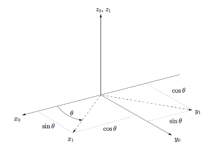 Figure 10: A rotation around the z-axis by angle $\theta$
Since they are also affine mappings, here are the matrices for rotations around the x-, y- and z-axis by angle $\theta$:
$$\begin{align*} \mathbf{R}_x(\theta) = \begin{pmatrix}1 & 0 & 0 \\ 0 & \cos(\theta) & -\sin(\theta) \\ 0 & \sin(\theta) & \cos(\theta)\end{pmatrix}, \mathbf{R}_y(\theta) = \begin{pmatrix}\cos(\theta) & 0 & \sin(\theta) \\ 0 & 1 & 0 \\ -\sin(\theta) & 0 & \cos(\theta)\end{pmatrix}, \mathbf{R}_z(\theta) = \begin{pmatrix}\cos(\theta) & -\sin(\theta) & 0 \\ \sin(\theta) & \cos(\theta) & 0 \\ 0 & 0 & 1\end{pmatrix} \end{align*}$$You can quite easily derive these matrices by geometric insight and the fact that the columns of the transformation matrix correspond to the transformed basis vectors of your coordinate system. So for a rotation around the z-axis by angle $\theta$ we get the following mappings of the basis vectors out of figure 10:
$$\begin{align*} \begin{pmatrix}1 \\ 0 \\ 0\end{pmatrix} \rightarrow \begin{pmatrix}\cos(\theta) \\ \sin(\theta) \\ 0\end{pmatrix}, \begin{pmatrix}0 \\ 1 \\ 0\end{pmatrix} \rightarrow \begin{pmatrix}-\sin(\theta) \\ \cos(\theta) \\ 0\end{pmatrix} \begin{pmatrix}0 \\ 0 \\ 1\end{pmatrix} \rightarrow \begin{pmatrix}0 \\ 0 \\ 1\end{pmatrix} \end{align*}$$As you can see the tree transformed basis vectors make up the transformation matrix. So the last thing we should know about rotations for now is that we are rotating counter-clockwise. This is because we are doing our transformations in a right hand coordinate system (we will come to the implications of that later).
Denavit-Hartenberg Description: Coordinate Systems
At that point, we got all we need to describe our robot using the Denavit-Hartenberg description. So how do we derive this description?
The basic idea is to assign a new coordinate system to every joint and then transform the coordinate system of one joint into the coordinate system of the next joint as we go along the robot until we reach the end effector. Since we want to have a fixed number of steps to transform one coordinate system into the next one, we will formulate some conditions which the coordinate systems have to meet:
Let $j_0, ..., j_n$ be the joints of the robot (either revolute or prismatic) and $\mathbf{x}_i, \mathbf{y}_i, \mathbf{z}_i$ be the vectors defining the coordinate system of $j_i$:
- $\mathbf{z}_i$ has to lie alongside the axis of movement of $j_i$
- $\mathbf{x}_{i+1}$ has to be orthogonal to $\mathbf{z}_i$ and $\mathbf{z}_{i+1}$ (choose $\mathbf{x}_0$ so that is it orthogonal to $\mathbf{z}_0$ and $\mathbf{z}_1$)
- $\mathbf{y}_i$ has to be choosen in such a way, that it forms a right hand coordinate system with $\mathbf{x}_i$ and $\mathbf{z}_i$
Allthough those constraints now look somewhat annoying they enable us to describe the transformation from one coordinate system into the other with just 4 values! So let's start with the easiest part - finding the $z_i$-axes of the joints in our SCARA robot. For that we only have to draw arrows through our joints:
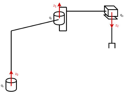 Figure 11: A sketch of the SCARA robot with the $\mathbf{z}_i$ vectors of the coordinate systems
Now in order to have a mathematical description of our $z_i$-axes let's assume that the robot is standing on an absolutely horizontal baseplate. With that we obtain $\mathbf{z}_0 = (0, 0, 1)^T$, $\mathbf{z}_1 = (0, 0, 1)^T$, $\mathbf{z}_2 = (0, 0, -1)^T$. So now that we have done that, we need to find the $x$-axes of the coordinate systems. Since $\mathbf{x}_i$ has to be orthogonal to $\mathbf{z}_i$ and $\mathbf{z}_{i-1}$ we should calculate $\mathbf{z}_i \times \mathbf{z}_{i-1}$ in order to find $\mathbf{x}_i$. If we do this in our case, we will always get $\mathbf{0}$ since $\mathbf{z}_0 \parallel \mathbf{z}_1 \parallel \mathbf{z}_2$. This basically means that there are infinitely many orthogonal vectors to choose from. So let's set $\mathbf{x}_0 = (1, 0, 0)^T$, $\mathbf{x}_1 = (\cos(q_1), \sin(q_1), 0)^T$ and $\mathbf{x}_2 = (\cos(q_1 + q_2), \sin(q_1 + q_2), 0)^T$. If we update our sketch accordingly we will get the following:
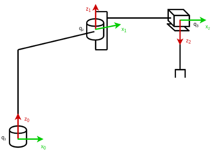 Figure 12: A sketch of the SCARA robot with the $\mathbf{x}_i$ and $\mathbf{z}_i$ vectors of the coordinate systems
We nearly got it! What's left are the $y_i$-axes. Since we assumed that the rotations will be done in a right hand coordinate system we need to ensure that we actually have one. To find $\mathbf{y}_i$, we will use the right hand rule, which is illustrated in the following picture:
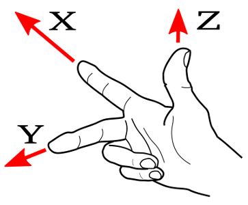 Figure 13: The right hand rule for finding the vectors $\mathbf{y}_i$ to form a right hand coordinate system
With the rule we should come to the conclusion that $\mathbf{y}_0 = (0, 1, 0)^T$, $\mathbf{y}_1 = (-\sin(q_1), \cos(q_1), 0)^T$ and $\mathbf{y}_2 = (-\sin(q_1 + q_2), \cos(q_1 + q_2), 0)^T$. So here is our final sketch of the coordinate frames:
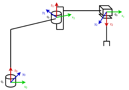 Figure 14: A sketch of the SCARA robot with the $\mathbf{x}_i$, $\mathbf{y}_i$ and $\mathbf{z}_i$ vectors of the coordinate systems
Denavit-Hartenberg Description: Transformations
So now that we have our coordinate system, we should worry about how to get from one to the other. In order to discuss this let's first add heights and lengths for the links of our SCARA robot:

Since we have that, let's try to get from the coordinate system of $j_0$ to the coordinate system of $j_1$. The first thing we need to do is make $\mathbf{x}_0$ and $\mathbf{x}_1$ parallel. For that we need a rotation around $\mathbf{z}_0$ by angle $q_1$. So our first transformation matrix looks like this:
$$\begin{align*} \text{Rot}(\mathbf{z}_0, \theta_1) = \begin{pmatrix}\cos(\theta_1) & -\sin(\theta_1) & 0 & 0 \\ \sin(\theta_1) & \cos(\theta_1) & 0 & 0 \\ 0 & 0 & 1 & 0 \\ 0 & 0 & 0 & 1\end{pmatrix}, \theta_1 = q_1 \end{align*}$$To see what's going on, here is the same sketch from above with the new coordinate system in dotted lines:

Now that we have this done, we are going to shift the coordinate system along the z-axis:
$$\begin{align*} \text{Trans}(\mathbf{z}_0, d_1) = \begin{pmatrix}1 & 0 & 0 & 0 \\ 0 & 1 & 0 & 0 \\ 0 & 0 & 1 & d_1 \\ 0 & 0 & 0 & 1\end{pmatrix}, d_1 = h_1 \end{align*}$$Again the sketch with the new coordinate system:

The third step is to shift the coordinate system along the x-axis so that we arrive at the same position where the coordinate system of the next joint has its base:
$$\begin{align*} \text{Trans}(\mathbf{x}_0, a_1) = \begin{pmatrix}1 & 0 & 0 & a_1 \\ 0 & 1 & 0 & 0 \\ 0 & 0 & 1 & 0 \\ 0 & 0 & 0 & 1\end{pmatrix}, a_1 = r_1 \end{align*}$$When we look at the following sketch, a question should arise:

The question is: Why should we need a fourth transformation? Well in this case we do not need it but if you look at the orientation of $\mathbf{z_1}$ and $\mathbf{z_2}$ you will notice that they point in the opposite direction. So the fourth transformation is a rotation around $x_0$ (by an angle of zero degree in this case):
$$\begin{align*} \text{Rot}(\mathbf{x}_0, \alpha_1) = \begin{pmatrix}1 & 0 & 0 & 0 \\ 0 & \cos(\alpha_1) & -\sin(\alpha_1) & 0 \\ 0 & \sin(\alpha_1) & \cos(\alpha_1) & 0 \\ 0 & 0 & 0 & 1\end{pmatrix}, \alpha_1 = 0 \end{align*}$$We now finish this transformation by multiplying the four matrices up so that we receive one transformation matrix which transforms the coordinate system of $j_0$ into the coordinate system of $j_1$:
$$\begin{align*} ^{0}T_1 &= \text{Rot}(\mathbf{z}_0, \theta_1) \text{Trans}(\mathbf{z}_0, d_1) \text{Trans}(\mathbf{x}_0, a_1) \text{Rot}(\mathbf{x}_0, \alpha_1) \\ &= \begin{pmatrix} \cos(\theta_1) & -\sin(\theta_1) \cos(\alpha_1) & \sin(\theta_1) \sin(\alpha_1) & a_1 \cos(\theta_1) \\ \sin(\theta_1) & \cos(\theta_1) \cos(\alpha_1) & -\cos(\theta_1) \sin(\alpha_1) & a_1 \sin(\theta_1) \\ 0 & \sin(\alpha_1) & \cos(\alpha_1) & d_1 \\ 0 & 0 & 0 & 1 \end{pmatrix} \end{align*}$$As you have probably already decuted, the general form of the transformation from the coordinate system of joint $j_{n-1}$ to the coordinate system of joint $j_{n}$ is:
$$\begin{align*} ^{n-1}T_n &= \text{Rot}(\mathbf{z}_{n-1}, \theta_n) \text{Trans}(\mathbf{z}_{n-1}, d_n) \text{Trans}(\mathbf{x}_{n-1}, a_n) \text{Rot}(\mathbf{x}_{n-1}, \alpha_n) \\ &= \begin{pmatrix} \cos(\theta_n) & -\sin(\theta_n) \cos(\alpha_n) & \sin(\theta_n) \sin(\alpha_n) & a_n \cos(\theta_n) \\ \sin(\theta_n) & \cos(\theta_n) \cos(\alpha_n) & -\cos(\theta_n) \sin(\alpha_n) & a_n \sin(\theta_n) \\ 0 & \sin(\alpha_n) & \cos(\alpha_n) & d_n \\ 0 & 0 & 0 & 1 \end{pmatrix} \end{align*}$$If you now wonder why we can be sure that those four transformations are enough the get from coordinate system to coordinate system then think about how we constructed the coordinate systems. Those constraints which we had to take care of there are now guaranteeing us that those four transformations are enough the get from one coordinate system to the next one. Consequently, you can be sure that you constructed the coordinate systems right if you are able to do the coordinate transformation with the four steps from above.
At this point I just want to add an example of the fourth transformation. We need this transformation when transforming the coordinate system from joint $j_1$ to the one of $j_2$. Here is a sketch of how it looks like:

Denavit-Hartenberg Description: Depiction
So as we saw, we only need the four parameters $\theta_n$, $d_n$, $a_n$ and $\alpha_n$ to describe the transformation from one coordinate system to the next. Consequently, we normally write them in a table. For our SCARA robot this table looks as follows:
| n | $\alpha_n$ | $a_n$ | $d_n$ | $\theta_n$ |
|---|---|---|---|---|
| 1 | 0 | $r_1$ | $h_1$ | $q_1$ |
| 2 | $\pi$ | $r_2$ | $h_2$ | $q_2$ |
| 3 | $\pi$ | 0 | $q_3$ | 0 |
The attentive among us may have noticed something. Since we have three transformations we need to have four coordinate systems. However, in our sketches we only had three. Let's fix this by adding the last coordinate system (which normally is the coordinate system of the task space):

From Denavit-Hartenberg to Forward Kinematics
At the beginning of the topic about Denavit-Hartenberg I promised that we would find an easy step-by-step approach to forward kinematics. But until now, we have only learned how to describe a robot in some fancy way. So how do we get from this description to our forward kinematics function $f(\mathbf{q})$? Luckily, this is quite easy, as we just have to do the following:
$$\begin{align*} f(\mathbf{q}) = ^0T_1 ... ^{n-1}T_n \mathbf{v}_0 \end{align*}$$The vector $\mathbf{v}_0$ is the position of joint $j_0$ in the task space (as a homogenous coordinate). So if was assume that our SCARA robot is positioned at $(0, 0, 0)^T$ we get the following forward kinematics function for it:
$$\begin{align*} f(\mathbf{q}) = ^0T_1 ^1T_2 ^{2}T_3 \begin{pmatrix}0 \\ 0 \\ 0 \\ 1\end{pmatrix} \end{align*}$$With this, we have talked enough about kinematics and will now move on to dynamics. Those wo want to do some calculus before moving to dynamics can now show that the Denavit-Hartenberg approach acutally leads to the same vector that we saw in the forward kinematics section.
Dynamics 
Getting the differential equations
All we need to know to build our model are the differential equations. We will consider two methods to get those.
Newton-Euler's Method
The Newton-Euler method is sometimes also referred to as force dissection. This method can be formalized nicely, however we will not do this here. The basic idea is to consider each joint independently from the rest of the system and calculate the resulting force on that joint by summing all individual forces. So lets do this for our robot.
We will start with the prismatic joint ($u_2$). Obviously this only depends on the second mass $m_2$. First we consider the forces along the axis of the cartisian space our robot lives in.
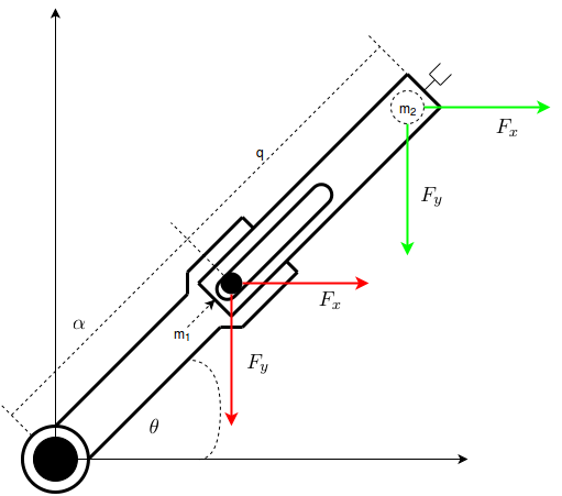 Figure 18. The forces acting on the mass are displayed in green. The resulting forces at the joint are displayed in red. Those forces are the same, just "shifted" to another location
To get those forces we first need the acceleration of that mass. We obtain this by differentiating the position two times with respect to the time. From the kinematics section we know
$$\begin{align*}
p_{x2} &= (\alpha+q) \cos(\theta) \\
p_{y2} &= (\alpha+q) \sin(\theta)
\end{align*}$$
hence
$$\begin{align*}
v_{x2} &= -(\alpha +q) \sin(\theta)\dot{\theta} + \dot{q}\cos(\theta) \\
v_{y2} &= (\alpha+q) \cos(\theta) \dot{\theta} + \dot{q}\sin(\theta)
\end{align*}$$
and
$$\begin{align*}
a_{x2} &= -(\alpha + q) \sin(\theta) \ddot{\theta} - (\alpha + q)\dot{\theta}^2\cos(\theta)- \sin(\theta)\dot{q}\dot{\theta} + \ddot{q}\cos(\theta) - \sin(\theta)\dot{\theta}\dot{q} \\ &= \left(-(\alpha + q)\ddot{\theta} - 2\dot{\theta}\dot{q}\right)\sin(\theta) + \left(\ddot{q} - (\alpha+q)\dot{\theta}^2\right)\cos(\theta) \\
a_{y2} &=(\alpha +q) \cos(\theta)\ddot{\theta} - (\alpha + q)\dot{\theta}^2\sin(\theta) + \cos(\theta)\dot{q}\dot{\theta} + \ddot{q}\sin(\theta) + \cos(\theta)\dot{\theta}\dot{q}\\
&= \left(\alpha +q)\ddot{\theta} + 2\dot{\theta}\dot{q} \right)\cos(\theta) + \left(\ddot{q} - (\alpha + q)\dot{\theta}^2\right)\sin(\theta)
\end{align*}$$
With this we can now compute the forces along each axis using Newton's second law of motion. Note that we also need to consider gravity, which acts along the $y$-axis
$$\begin{align*}
m_2 \left[\left(-(\alpha + q)\ddot{\theta} - 2\dot{\theta}\dot{q}\right)\sin(\theta) + \left(\ddot{q} - (\alpha+q)\dot{\theta}^2\right)\cos(\theta)\right] &= F_{x2} \\
m_2 \left[\left(\alpha +q)\ddot{\theta} + 2\dot{\theta}\dot{q} \right)\cos(\theta) + \left(\ddot{q} - (\alpha + q)\dot{\theta}^2\right)\sin(\theta)\right] &= F_{y2} - m_2 g
\end{align*}$$
Now we have the forces along the axis. However we are interested in the forces in the reference frame of the robot. To get those we need to rotate by $\theta$. Note that we rotate clockwise and hence invert the rotationmatrix.
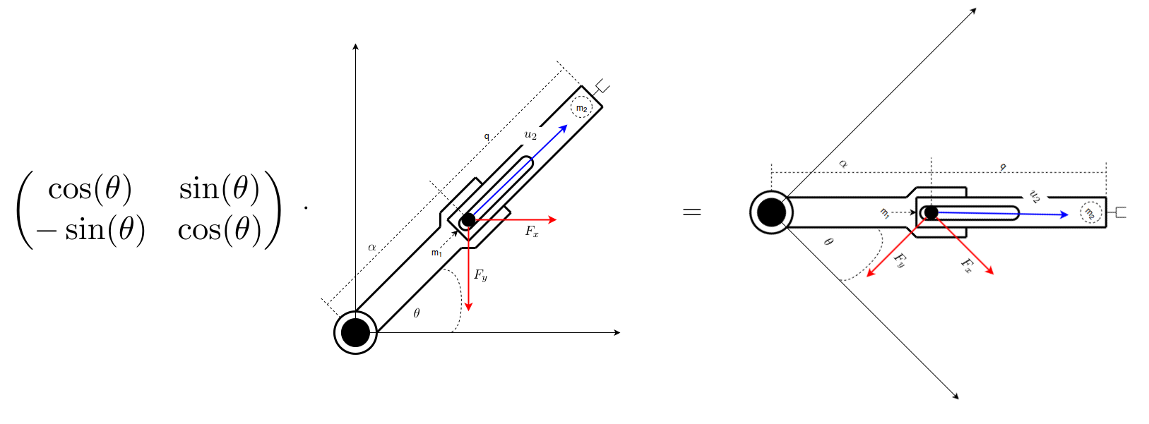 Figure 19. We multiply all forces with the rotation matix to get in the robot's reference frame
For $u_2$ this yields $$\begin{align*} u_2&=F_{x} \cos(\theta) + F_{y}\sin(\theta) \\ \end{align*}$$ All we need to do now is plug in the values $$\begin{align*} u_2&=m_2 \left[\left(-(\alpha + q)\ddot{\theta} - 2\dot{\theta}\dot{q}\right)\sin(\theta) + \left(\ddot{q} - (\alpha+q)\dot{\theta}^2\right)\cos(\theta)\right] \cos(\theta) \\ &+ m_2 \left[\left(\alpha +q)\ddot{\theta} + 2\dot{\theta}\dot{q} \right)\cos(\theta) + \left(\ddot{q} - (\alpha + q)\dot{\theta}^2\right)\sin(\theta)\right] \sin(\theta) + m_2 g \sin(\theta) \\ &= m_2\left[\left(-(\alpha + q)\ddot{\theta} - 2\dot{\theta}\dot{q}\right)\sin(\theta)\cos(\theta) + \left(\ddot{q} - (\alpha+q)\dot{\theta}^2\right)\cos^2(\theta)\right] \\ &+ m_2\left[\left(\alpha +q)\ddot{\theta} + 2\dot{\theta}\dot{q} \right)\cos(\theta)\sin(\theta) + \left(\ddot{q} - (\alpha+q)\dot{\theta}^2\right)\sin^2(\theta)\right] \\ &+ m_2 g \sin(\theta) \\ &=m_2 \ddot{q} - m_2(\alpha+q)\dot{\theta}^2 + m_2 g \sin(\theta) \end{align*}$$
Now we do the same for the rotary joint ($u_1$). This time we need to consider both masses $m_1$ and $m_2$.
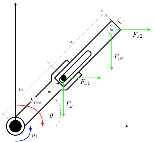 Figure 20. Forces acting on masses are displayed in green. For the resulting force (red) we need to consider the length of the leverage arms. Out motor force (blue) acts against the resulting force
We will do this seperatly, starting with $m_1$. Again we need to compute the acceleration first.
$$\begin{align*}
p_{x1} &= \cos(\theta) \alpha \\
p_{y1} &= \sin(\theta) \alpha \\
v_{x1} &= -\alpha\sin(\theta)\dot{\theta}\\
v_{y1} &= \alpha\cos(\theta)\dot{\theta} \\
a_{x1} &= -\alpha\left(\sin(\theta)\ddot{\theta} + \cos(\theta)\dot{\theta}^2\right)\\
a_{y1} &= \alpha\left(\cos(\theta)\ddot{\theta} - \sin(\theta)\dot{\theta}^2\right)
\end{align*}$$
Next, again with the help of our friend Newton, we obtain the forces along the axis. That guy really deserves a snickers. Note however that $m_1$ has a leverage arm of length $\alpha$. This needs to be considered too.
$$\begin{align*}
-m_1\alpha \alpha\left(\sin(\theta)\ddot{\theta} + \cos(\theta)\dot{\theta}^2\right) &= F_{x1} \\
m_1\alpha \alpha\left(\cos(\theta)\ddot{\theta} - \sin(\theta)\dot{\theta}^2\right) &= F_{y1} - m_1 \alpha g \\
\end{align*}$$
Again, to get in the right reference frame we need to rotate
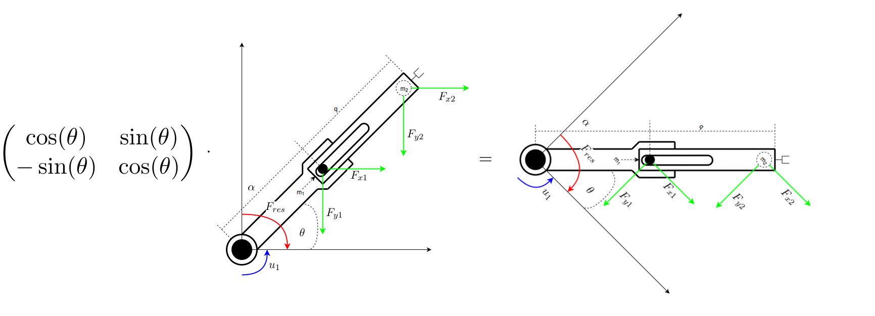 Figure 21. We multiply all forces with the rotation matix to get in the robot's reference frame
This yields
$$\begin{align*}
u_{11} =& -F_{x1} \sin(\theta) + F_{y1} \cos(\theta) \\
u_{12} =& - F_{x2} \sin(\theta) + F_{y2} \cos(\theta) \\
\end{align*}$$
Hence for $u_{11}$ we get
$$\begin{align*}
u_{11} =& m_1\alpha^2 \left[\left(\sin(\theta)\ddot{\theta} + \cos(\theta)\dot{\theta}^2\right) \right] \sin(\theta) + m_1\alpha^2 \left[\left(\cos(\theta)\ddot{\theta} - \sin(\theta)\dot{\theta}^2\right) \right] \cos(\theta)
\\ &+ m_1 \alpha g \cos(\theta)\\
=& m_1\alpha^2 \left(\sin^2(\theta)\ddot{\theta} + \sin(\theta)\cos(\theta)\dot{\theta}^2\right) + m_1\alpha^2 \left(\cos^2(\theta)\ddot{\theta} - \cos(\theta)\sin(\theta)\dot{\theta}^2\right)
\\ &+ m_1 \alpha g \cos(\theta) \\
=& m_1\alpha^2 \ddot{\theta} + m_1 \alpha g \cos(\theta). \\
\end{align*}$$
For the second mass we already know the acceleration. Again to calculate the force we have to consider the leverage arm, this time of length $(\alpha + q)$
$$\begin{align*}
m_2(\alpha + q) \left[ \left(-(\alpha + q)\ddot{\theta} - 2\dot{\theta}\dot{q}\right)\sin(\theta) + \left(\ddot{q} - (\alpha+q)\dot{\theta}^2\right)\cos(\theta) \right] &= F_{x2} \\
m_2(\alpha + q) \left[ \left(\alpha +q)\ddot{\theta} + 2\dot{\theta}\dot{q} \right)\cos(\theta) + \left(\ddot{q} - (\alpha + q)\dot{\theta}^2\right)\sin(\theta) \right] &= F_{y2} -m_2(\alpha+q) g
\end{align*}$$
The rotation yields
$$\begin{align*}
u_{12}=&m_2(\alpha+q) \left[ \left((\alpha + q)\ddot{\theta} + 2\dot{\theta}\dot{q}\right)\sin(\theta) - \left(\ddot{q} - (\alpha+q)\dot{\theta}^2\right)\cos(\theta)\right] \sin(\theta)\\
+& m_2(\alpha + q) \left[ \left((\alpha +q)\ddot{\theta} + 2\dot{\theta}\dot{q} \right)\cos(\theta) + \left(\ddot{q} - (\alpha + q)\dot{\theta}^2\right)\sin(\theta) \right] \cos(\theta) \\
+& m_2(\alpha+q) g \cos(\theta)\\
=&m_2(\alpha+q) \left[ \left((\alpha + q)\ddot{\theta} + 2\dot{\theta}\dot{q}\right)\sin^2(\theta) - \left(\ddot{q} -(\alpha+q)\dot{\theta}^2\right)\sin(\theta)\cos(\theta)\right] \\
+& m_2(\alpha + q) \left[ \left((\alpha +q)\ddot{\theta} + 2\dot{\theta}\dot{q} \right)\cos^2(\theta) + \left(\ddot{q} - (\alpha + q)\dot{\theta}^2\right)\cos(\theta) \sin(\theta) \right] \\
+& m_2(\alpha+q) g \cos(\theta)\\
=& m_2(\alpha + q)^2\ddot{\theta} + 2m_2(\alpha + q)\dot{\theta}\dot{q} + m_2(\alpha+q) g \cos(\theta)
\end{align*}$$
To get the total force acting on the first joint we know just need to add
$$\begin{align*}
u_1 &= u_{11} + u_{12}\\
&= m_1\alpha^2 \ddot{\theta} + m_1 \alpha g \cos(\theta) + m_2(\alpha + q)^2\ddot{\theta} + 2m_2(\alpha + q)\dot{\theta}\dot{q} + m_2(\alpha+q) g \cos(\theta)\\
&= \left(m_1\alpha^2 + m_2(\alpha + q)^2\right) \ddot{\theta} + 2m_2(\alpha + q)\dot{\theta}\dot{q} + \left(m_1\alpha + m_2(\alpha + q)\right)g \cos(\theta)
\end{align*}$$
We can now write this in the martix form shwon above
Figure 21. We multiply all forces with the rotation matix to get in the robot's reference frame
This yields
$$\begin{align*}
u_{11} =& -F_{x1} \sin(\theta) + F_{y1} \cos(\theta) \\
u_{12} =& - F_{x2} \sin(\theta) + F_{y2} \cos(\theta) \\
\end{align*}$$
Hence for $u_{11}$ we get
$$\begin{align*}
u_{11} =& m_1\alpha^2 \left[\left(\sin(\theta)\ddot{\theta} + \cos(\theta)\dot{\theta}^2\right) \right] \sin(\theta) + m_1\alpha^2 \left[\left(\cos(\theta)\ddot{\theta} - \sin(\theta)\dot{\theta}^2\right) \right] \cos(\theta)
\\ &+ m_1 \alpha g \cos(\theta)\\
=& m_1\alpha^2 \left(\sin^2(\theta)\ddot{\theta} + \sin(\theta)\cos(\theta)\dot{\theta}^2\right) + m_1\alpha^2 \left(\cos^2(\theta)\ddot{\theta} - \cos(\theta)\sin(\theta)\dot{\theta}^2\right)
\\ &+ m_1 \alpha g \cos(\theta) \\
=& m_1\alpha^2 \ddot{\theta} + m_1 \alpha g \cos(\theta). \\
\end{align*}$$
For the second mass we already know the acceleration. Again to calculate the force we have to consider the leverage arm, this time of length $(\alpha + q)$
$$\begin{align*}
m_2(\alpha + q) \left[ \left(-(\alpha + q)\ddot{\theta} - 2\dot{\theta}\dot{q}\right)\sin(\theta) + \left(\ddot{q} - (\alpha+q)\dot{\theta}^2\right)\cos(\theta) \right] &= F_{x2} \\
m_2(\alpha + q) \left[ \left(\alpha +q)\ddot{\theta} + 2\dot{\theta}\dot{q} \right)\cos(\theta) + \left(\ddot{q} - (\alpha + q)\dot{\theta}^2\right)\sin(\theta) \right] &= F_{y2} -m_2(\alpha+q) g
\end{align*}$$
The rotation yields
$$\begin{align*}
u_{12}=&m_2(\alpha+q) \left[ \left((\alpha + q)\ddot{\theta} + 2\dot{\theta}\dot{q}\right)\sin(\theta) - \left(\ddot{q} - (\alpha+q)\dot{\theta}^2\right)\cos(\theta)\right] \sin(\theta)\\
+& m_2(\alpha + q) \left[ \left((\alpha +q)\ddot{\theta} + 2\dot{\theta}\dot{q} \right)\cos(\theta) + \left(\ddot{q} - (\alpha + q)\dot{\theta}^2\right)\sin(\theta) \right] \cos(\theta) \\
+& m_2(\alpha+q) g \cos(\theta)\\
=&m_2(\alpha+q) \left[ \left((\alpha + q)\ddot{\theta} + 2\dot{\theta}\dot{q}\right)\sin^2(\theta) - \left(\ddot{q} -(\alpha+q)\dot{\theta}^2\right)\sin(\theta)\cos(\theta)\right] \\
+& m_2(\alpha + q) \left[ \left((\alpha +q)\ddot{\theta} + 2\dot{\theta}\dot{q} \right)\cos^2(\theta) + \left(\ddot{q} - (\alpha + q)\dot{\theta}^2\right)\cos(\theta) \sin(\theta) \right] \\
+& m_2(\alpha+q) g \cos(\theta)\\
=& m_2(\alpha + q)^2\ddot{\theta} + 2m_2(\alpha + q)\dot{\theta}\dot{q} + m_2(\alpha+q) g \cos(\theta)
\end{align*}$$
To get the total force acting on the first joint we know just need to add
$$\begin{align*}
u_1 &= u_{11} + u_{12}\\
&= m_1\alpha^2 \ddot{\theta} + m_1 \alpha g \cos(\theta) + m_2(\alpha + q)^2\ddot{\theta} + 2m_2(\alpha + q)\dot{\theta}\dot{q} + m_2(\alpha+q) g \cos(\theta)\\
&= \left(m_1\alpha^2 + m_2(\alpha + q)^2\right) \ddot{\theta} + 2m_2(\alpha + q)\dot{\theta}\dot{q} + \left(m_1\alpha + m_2(\alpha + q)\right)g \cos(\theta)
\end{align*}$$
We can now write this in the martix form shwon above
 Figure 22. Left: Sir Isaac Newton with his well deserved snickers. Right: Joseph-Louis Lagrange
Lagrangian Method
The Lagrangian Method is a completely different approach. In order to use it we first have to consider potential and kinetic energy. We know them from high school so here we will just shortly recapture the formulas and derive the energies for our robot.
Potential Energy
The general formula for potential energy (at least in mechanics) is given by
$$\begin{align*}
P = m g h.
\end{align*}$$
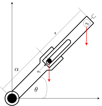 Figure 23. Gravity acting on the robot
We only need to consider the distance from the point masses to the table our robot is mounted on. Considering both masses separately we get $$\begin{align*} p_1 &= m_1 g \alpha\sin(\theta)\\ p_2 &= m_2 g (\alpha + q) \sin(\theta)\\ p &= p_1 +p_2 \end{align*}$$
Kinetic Energy
The general formula for kinetic energy is given by
$$\begin{align*}
K = \frac{1}{2}m v^2
\end{align*}$$
where $v$ denotes the velocity of the mass under consideration. Again we consider the masses separately.
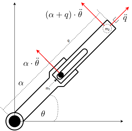 Figure 24. Velocities of the masses
For $m_1$ we get $$\begin{align*} k_1 &= \frac{1}{2}m_1 \left(\dot{\theta} \alpha \right)^2\\ &= \frac{1}{2}m_1 \dot{\theta}^2 \alpha^2 \end{align*}$$ For $m_2$ we need to consider both velocities acting on the mass. Thus $$\begin{align*} k_2 &= \frac{1}{2}m_2 \left(\alpha +q)\dot{\theta}\right)^2 + \frac{1}{2}m_2 \dot{q} \\ &= \frac{1}{2}m_2\left((\alpha + q)^2\dot{\theta}^2 + \dot{q}^2\right) \\ \end{align*}$$ To get the total kinetic energy we just sum up $$\begin{align*} k &= k_1 + k_2. \end{align*}$$
Langrangian Equation
Now that we know about the potential and kinematic energy we can use them to get the equation for our dynamics model. Lagrange stated that we can do so by using the following equation
$$\begin{align*}
u_i = \dfrac{d}{dt}\dfrac{\partial L}{\partial \dot{q_i}} - \dfrac{\partial L}{\partial q_i}
\end{align*}$$
where $L$ is given by
$$\begin{align*}
L = K - P.
\end{align*}$$
It can be proven that this is valid for all dynamic systems, to see why you need to sacrifice a goat to an old guy with funny hairstyle, or just look it up on Wikipedia, however do not blame me if you cry afterwards.
All we need to do now is plug our values for the energies into the equation. In our case $L$ is given by
$$\begin{align*}
L = \frac{1}{2}m_1\alpha^2\dot{\theta}^2 + \frac{1}{2}m_2\left((\alpha + q)^2\dot{\theta}^2 + \dot{q}^2\right) - m_1 \alpha g \sin(\theta) - m_2 (\alpha + q) g \sin(\theta)
\end{align*}$$
We will calculate for the rotary joint first. For the first part of the right sight of the equation we need to differentiate with respect to the velocity.
$$\begin{align*}
\dfrac{\partial L}{ \partial \dot{\theta}} &= m_1 \alpha^2 \dot{\theta} + m_2 (\alpha +q)^2 \dot{\theta} \\
\dfrac{d}{dt} \dfrac{\partial L}{ \partial \dot{\theta}} &= m_1 \alpha^2 \ddot{\theta} + m_2 (\alpha +q)^2 \ddot{\theta} + 2 m_2 (\alpha + q) \dot{q} \dot{\theta}\\
&= \left(m_1 \alpha^2 + m_2(\alpha + q)^2\right) \ddot{\theta} + 2 m_2( \alpha + q) \dot{\theta} \dot{q}
\end{align*}$$
For the second part of the right sight we differentiate with respect to the position.
$$\begin{align*}
\dfrac{\partial L}{ \partial \theta} &= - m_1 \alpha g \cos(\theta) - m_2 (\alpha + q) g \cos(\theta) \\
&= - \left(m_1 \alpha + m_2 (\alpha + q)\right) g \cos(\theta)
\end{align*}$$
Pluging this in we get
$$\begin{align*}
\dfrac{d}{dt} \dfrac{\partial L}{ \partial \dot{\theta}} - \dfrac{\partial L}{\partial \theta} &= \left(m_1 \alpha^2 + m_2(\alpha + q)^2\right) \ddot{\theta} + 2 m_2( \alpha + q) \dot{\theta} \dot{q} + \left(m_1 \alpha + m_2 (\alpha + q)\right) g \cos(\theta) \\
u_1 &= \left(m_1 \alpha^2 + m_2(\alpha + q)^2\right) \ddot{\theta} + 2 m_2( \alpha + q) \dot{\theta} \dot{q} + \left(m_1 \alpha + m_2 (\alpha + q)\right) g \cos(\theta)
\end{align*}$$
Now we do the same for the prismatic joint.
$$\begin{align*}
\dfrac{\partial L}{ \partial \dot{q}} &= m_2 \dot{q} \\
\dfrac{d}{dt}\dfrac{\partial L}{d \partial \dot{q}} &= m_2 \ddot{q} \\
\dfrac{\partial L}{ \partial q} &= m_2(\alpha + q) \dot{\theta}^2 - m_2g\sin(\theta) \\
\dfrac{d}{dt} \dfrac{\partial L}{ \partial \dot{q}} - \dfrac{\partial L}{\partial q} &= m_2 \ddot{q} - m_2(\alpha + q) \dot{\theta}^2 + m_2g\sin(\theta) \\
u_2 &= m_2 \ddot{q} - m_2(\alpha + q) \dot{\theta}^2 + m_2g\sin(\theta)
\end{align*}$$
We directly get the equation for the inverse dynamics model which can be written in the matrix form again:
You should also note that we get the same result as we got using force dissection (which is nice and makes me very happy - or I got both wrong)
Comparison of Complexity
Naturally the question arises which method to use. Considering this theoretically Newton-Euler is in $\mathcal{O}(n)$ while the Lagrangian is in $\mathcal{O}(n^3)$ so the answer should be clear and if need performance, it is. However it is still good to know about both, since, as seen in the example above, often the Lagrangian is faster if you do the calculations for a robot by hand, especially if you have no clue about physics.